Senior Design · Wabtec rail efficiency study

AI Drivetrain Efficiency

Machine learning for smarter locomotive motor power distribution.

Michael Penfield · Joel Sander · Connor Pflugh · Jacob Harsch

Penn State Behrend Wabtec Corporation

Introduction

Wabtec builds and maintains locomotives that run in demanding environments.

  • Global rail equipment, systems, and digital solutions provider.
  • High-performance locomotives operate around the clock.
  • Sustainability gains matter when multiplied across fleets.
Wabtec locomotive render

Needs · Problem Illustrated

Even power splits assume every traction motor behaves the same.

Wear and operating conditions can make one motor less efficient than another.

Input1000 W
166W166W166W166W166W166W
150 kN120 kN140 kN130 kN140 kN145 kN
Total output: 825 kN

Needs · AI Distribution

AI can shift the split toward motors that waste less power.

The model reads per-motor losses and returns a custom allocation.

AI split1000 W
100W250W300W150W100W100W
140 kN150 kN135 kN140 kN140 kN145 kN
Total output: 850 kN

Project Goal

Run a feasibility study for machine-learning-driven motor power distribution.

Objective

Find a suitable model for long-term efficiency gains.

Constraint

No real-world drivetrain dataset, so data is simulated.

Success

Show gains on scenarios the model never saw during training.

Our Approach

Simulate, train, compare.

  • 1Simulate train behavior.
  • 2Train AI models on generated scenarios.
  • 3Compare performance to an even-split baseline.
5,000scenarios
100time steps each
10 secsampling
-2% to +3%track slope

The Simulation

A virtual locomotive environment creates the learning signal.

Each motor receives a loss factor at scenario start, then the train advances through time.

Track slope Weight Throttle Motor losses Loss = motor power × loss factor

Model Setup

Input losses. Output power fractions.

The action must distribute all available power without giving everything to one motor.

Reward (baseline loss − AI loss) ÷ baseline loss

Positive when the AI beats the even split.

How the AI Learns

Trial, measure, adjust.

Try

Choose a distribution.

Measure

Compare efficiency to baseline.

Adjust

Update the policy toward better choices.

Models Tested

Five candidates covered memory, control, stability, and a supervised baseline.

Q-TableSARSADDPGTD3MLP

Why Multiple Models?

Different algorithms fail for different reasons.

Learning style

Discrete memory vs. continuous control.

Complexity

Some models handle noisy scenarios better.

Stability

Variance and convergence decide whether a result is usable.

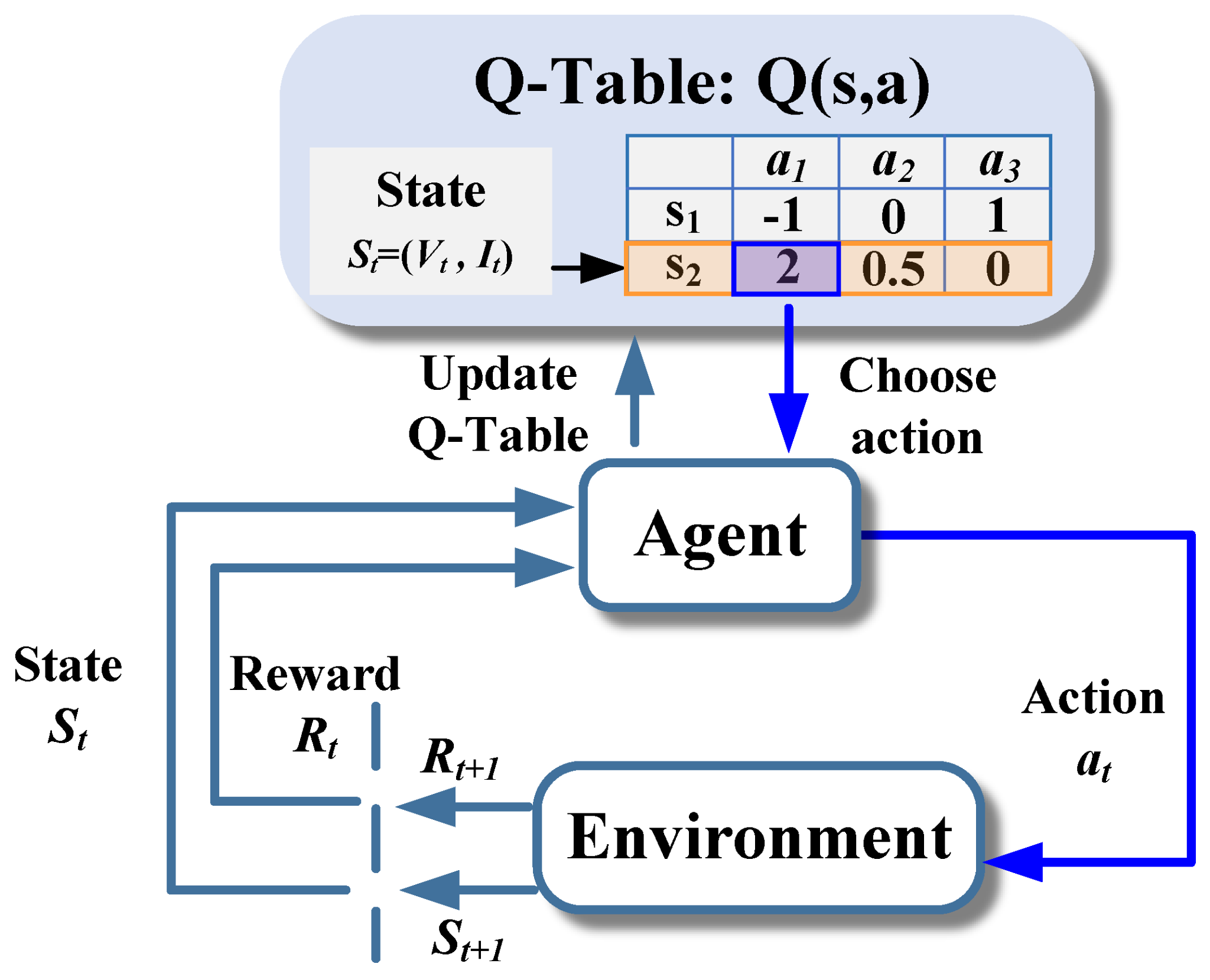
State-Based Candidates

Q-Table and SARSA make discrete policy jumps.

  • Q-Table remembers best actions for known states.
  • SARSA behaves more conservatively.
  • Both struggle when smooth control is needed.
Q-table reinforcement learning diagram

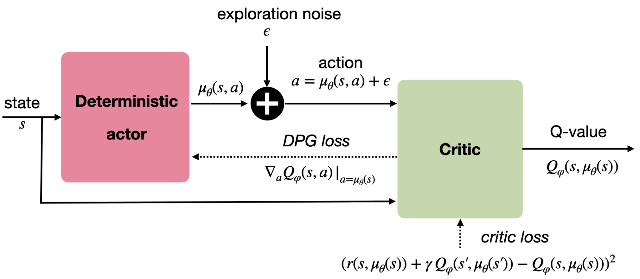
Continuous Candidates

DDPG and TD3 treat power allocation like dimmer switches.

  • Actor chooses the power setting.
  • Critic evaluates the choice.
  • TD3 adds a second critic for stability.
DDPG actor critic flow diagram

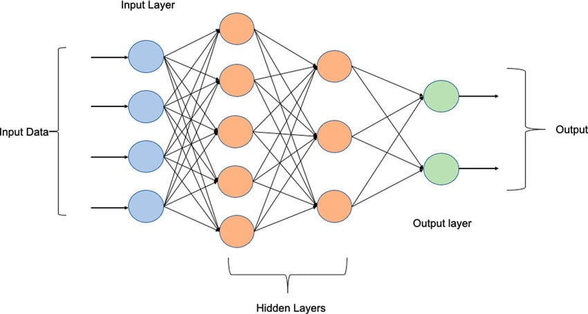
Supervised Learning Check

MLP tested whether reinforcement learning was the right paradigm.

Labels were generated from the simulation equations using KKT optimization.

Multilayer perceptron diagram

Smarter Training

Parallel learners compare results and keep the best ideas.

Multiple versions of the same model run at once, flushing out weak moves faster.

Model 1Model 2Model 3 Shared policy

Training Strategy · Metaheuristic

Segment learning blends local discoveries into a global update.

Phase 1

Learn smaller training segments first.

Phase 2

Blend segment scores like pheromones.

Phase 3

Train globally with old and new information.

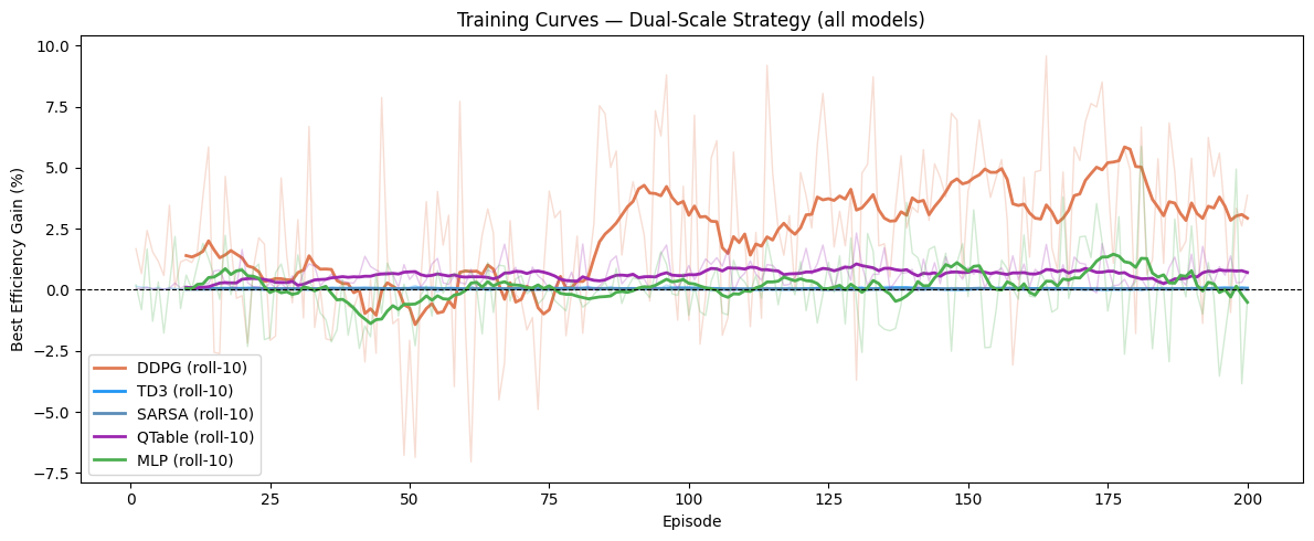
Best Performance Model

DDPG generalized after roughly 75 training episodes.

The orange line showed stronger gains, though variance suggests more training would help consistency.
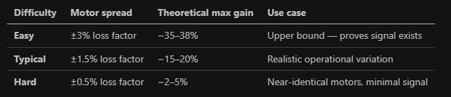
Training scores chart

Result Validation

Models were tested against new difficulty levels.

Each difficulty scales motor inefficiency to create easier or harder validation sets.

Validation difficulty table

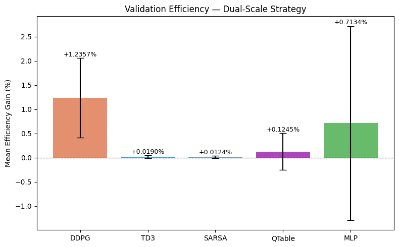
Final Results · Validation

DDPG consistently achieved the strongest validation results.

  • Some models failed to converge.
  • Others had too much variance.
  • DDPG scaled across easy, medium, and hard cases.
Validation efficiency comparison

Estimated Financial Impact

Small gains become meaningful across a fleet.

Validated gain+1.24%
Per locomotive$7,440
Fleet fuel saved2.48M gal
Fleet savings$7.44M
Industry baseline ~200,000 gal

Annual fuel per line-haul locomotive

$600,000

Baseline annual fuel cost per locomotive

AI advantage +1.24%

Validated efficiency gain in a typical variation scenario

$7,440

Annual savings per locomotive

1,000 locomotive fleet 2.48M gal

Total annual fuel reduction

$7.44M

Total annual cost savings

Thank You

AI-guided power distribution is feasible, measurable, and worth deeper validation.

Next step: move from simulated losses to richer drivetrain data and real operating profiles.